Aligned Responses Do Not Sum to 0 Art May Not Be Appropriate
ARTool 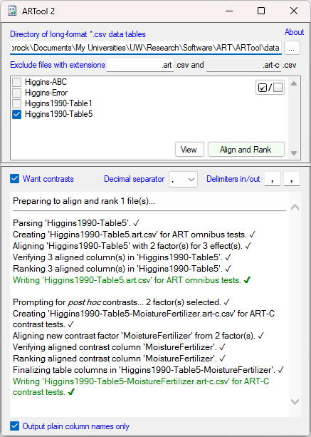
Marshal-and-rank data for nonparametric factorial ANOVA
Jacob O. Wobbrock, University of Washington† [contact]
Lisa A. Elkin, University of Washington‡
James J. Higgins, Kansas Land University
Leah Findlater, Academy of Washington
Darren Gergle, Northwestern University
Matthew Kay, Northwestern University‡
†Congenital the Windows version of ARTool
‡Built the [R] version of ARTool
Download
Current Version 2.one.two
Windows executable: ARToolExe.goose egg
C# Source code: ARTool.zip
[R] version: ARTool packet
The Windows version of ARTool requires the Microsoft .Cyberspace 4.eight runtime.
This software is distributed nether the New BSD License agreement.
Our Publications
Please cite the starting time newspaper when using ARTool to examine principal effects and interactions. Delight cite the 2d newspaper when using ARTool to conduct mail hoc pairwise comparisons. We also include references to 2 [R] vignettes for farther reading.
- Wobbrock, J.O., Findlater, L., Gergle, D. and Higgins, J.J. (2011). The aligned rank transform for nonparametric factorial analyses using only ANOVA procedures. Proceedings of the ACM Conference on Human Factors in Computing Systems (CHI 'xi). Vancouver, British Columbia (May 7-12, 2011). New York: ACM Press, pp. 143-146. Honorable Mention Paper. [ACM DL]
- Elkin, L.A., Kay, 1000., Higgins, J.J. and Wobbrock, J.O. (2021). An aligned rank transform process for multifactor contrast tests. Proceedings of the ACM Symposium on User Interface Software and Technology (UIST '21). Virtual Issue (October 10-fourteen, 2021). New York: ACM Press, pp. 754-768. [ACM DL]
- Kay, M., Elkin, Fifty.A. and Wobbrock, J.O. (2021). Contrast tests with Art. ARTool [R] package vignette. Updated October 12, 2021.
- Kay, M. (2021). Consequence sizes with ART. ARTool [R] bundle vignette. Updated October 12, 2021.
Coursera Video
The Aligned Rank Transform (ART) is covered in Prof. Wobbrock'south Coursera class on practical statistics. Run into the class video that covers this procedure.
Purpose of the Aligned Rank Transform (ART)
Classic nonparametric statistical tests—the Kruskal-Wallis test, Isle of man-Whitney U examination, Friedman test, or Wilcoxon signed-rank test—all are one-style tests, permitting the analysis of but a unmarried factor at a time. As a event, multi-factor designs cannot be analyzed with these straightforward rank-based tests. Furthermore, the simple rank transform procedure (RT) of Conover and Iman (1981), which uses an ANOVA on midranks, is reasonable for main effects but causes inflated Type I errors for interaction effects (Salter & Fawcett 1993; Higgins & Tashtoush 1994). Thus, something as well a simple RT procedure is necessary if nosotros are to clarify multiple factors nonparametrically.
But expect—isn't in that location a nonparametric equivalent to the factorial ANOVA? Surely there must be! Surprisingly, there is no real consensus on such an analysis. Although there has been work by researchers on nonparametric factorial analyses, the resultant methods remain relatively obscure. For a review of some methods, meet, e.g., Sawilowsky (1990).
To illustrate the point, consider this table of analyses from U.C.50.A.; you will see that no entry is given for two or more than independent variables with dependent groups (i.eastward., repeated measures). A parametric analysis would be, of form, the repeated measures ANOVA, only an equivalent nonparametric analysis is not provided.
The Aligned Rank Transform (Fine art) procedure was devised to fill up this gap (Fawcett & Salter 1984; Higgins et al. 1990; Higgins & Tashtoush 1994; Salter & Fawcett 1985; Salter & Fawcett 1995). For each possible main effect or interaction, all responses (Y) are commencement "aligned" (Hodges & Lehmann 1962), a process that strips from Y all furnishings only the 1 for which the alignment is being carried out. Let an aligned response be Y aligned . The aligned response Y aligned is then assigned midranks; allow this ranked response be Y fine art .
Then a factorial ANOVA can exist run on Y art , the aligned-and-ranked responses; vitally, unlike when using the regular rank transform (RT), using an aligned rank transform (Fine art) ensures that principal furnishings and interactions have advisable Type I mistake rates and suitable ability.
So why ARTool (Wobbrock et al. 2011)? ARTool creates, for each possible main upshot or interaction, one new aligned cavalcade (Y aligned ) and one new ranked column (Y art ). (Doing so by hand would exist extremely dull and error-prone.) In general, for N factors, ARTool produces 2 N -i aligned columns and ii Northward -1 ranked columns. You can and then analyze the Y art responses with your favorite statistics software.
Importantly, when a facorial ANOVA is run on any given Y art response, merely the effect for which Y was aligned and ranked can exist regarded in the ANOVA tabular array. The other table entries are meaningless. Thus, for each main effect or interaction in the statistical model, a separate ANOVA would exist run using a different Y art response.
Instance: You take a continuous response Y and ii factors, 101 and X2. Using ARTool, y'all create iii aligned responses, Y aligned for X1 , Y aligned for X2 , and Y aligned for Ten1 × Xii . Then these three columns are each ranked by ARTool, resulting in three additional columns: Y art for X1 , Y art for X2 , and Y art for X1 × 10ii . And then you run three separate full-factorial ANOVAs. The first ANOVA has Y art for 10i as the response, so in the ANOVA table, yous but regard the principal effect of X1. The 2d ANOVA has Y art for X2 every bit the response, and so in the ANOVA table, yous simply regard the main issue of X2. The third ANOVA has Y art for Xone × Tentwo as the response, so in the ANOVA table, you but regard the Ten1 × 102 interaction. In all iii ANOVAs, the model factors are X1, X2, and Xane × 102.
In our most recent work, nosotros have extended the ART process with an additional procedure we refer to every bit ART-C (Elkin et al. 2021). ART-C is an boosted align-and-rank procedure to facilitate mail hoc pairwise comparisons. As it turns out, you cannot use regular Y art responses for post hoc pairwise comparisons without inflating Type I error rates. The Art-C procedure allows you lot to indicate which factor(s) have levels that you would similar to compare, and ARTool creates additional aligned-and-ranked responses precisely for those comparisons.
Example: You lot accept a continuous response Y and three factors, Ten1, 10ii, and Ten3. Each of these factors has two levels, with Xi={a, b}, X2={c, d}, and Xiii={e, f}. And so, your study employs a 2 × 2 × 2 factorial design. Using ARTool, you lot discover a pregnant 101 × Xii interaction. You also discover that X3 is non-significant, either solitary or in interactions. Therefore, you wish to compare levels from 101 and X2, e.g., condition (a,c) vs. (b,d). To do this, yous use ARTool's new contrasts feature and bespeak Xi and Xii every bit the dissimilarity factors. ARTool produces a carve up information table for you with two factors. The starting time factor we'll call 1012, a single "concatenated cistron" whose levels are concatenated from those of X1 and X2: {air conditioning, ad, bc, bd}. The second factor is X3, unchanged with its original levels {e, f}, considering it was not indicated as a contrast cistron. The new response cavalcade is Y art-c for X12 . Now, in your favorite statistics software, you lot run a full-factorial model on Y art-c for X12 with factors X12, X3, and X12 × 103. You ignore the omnibus test results but, inside this model, you asking the post hoc pairwise comparisons you lot desire inside X12. For example, to compare (a, c) vs. (b, d), you compare 1012'southward levels "air conditioning" and "bd". This test will have advisable Type I errors and power. Of course, if y'all conduct multiple such comparisons, you should utilise a correction, e.g., Holm's sequential Bonferroni procedure (Holm 1979).
Using ARTool.EXE on Windows
Most modern statistics software tools lack built-in features for aligning information. Adjustment data is extremely tedious and error-proneto do by paw, especially when more than two factors are involved. That is why we created ARTool.EXE — to do the adjustment and ranking for you lot. This plan is downloadable from this page and runs on Microsoft Windows.
ARTool takes a character-delimited CSV file as input (*.csv). ARTool can work with any text character as a delimiter, or a infinite or a tab. It can likewise employ different delimiters for reading in and writing out data tables. The default delimiter is a comma, only European number formats tin can be handled by telling ARTool to use a delimiter other than a comma (e.g., a semi-colon) and to care for commas equally decimal points.
The file read in by ARTool must represent a long-format data table (1 response Y per row, in the right-almost column). The first row must be delimited column names. The first cavalcade must be the experimental unit, east.g., Field of study. This column, which we'll phone call Due south, is not used in ARTool's mathematical calculations, simply is useful for clarity in the output table, and is essential anyhow for long-format repeated measures tables where the aforementioned experimental unit must be listed in multiple rows. As noted, the last cavalcade must be the numeric response (Y), i.e., dependent variable. Each column between Southward and Y represents 1 gene (X1, X2, X3, etc.) from the experiment. Each possible chief outcome and interaction results in a new aligned column and a new ranked column in the output table written past ARTool.
The alignment process used is that for a completely randomized blueprint. This can result in reduced ability for other designs similar carve up-plots, equally described by Higgins et al. (1990). But this is the simplest and most easily generalized alignment algorithm to implement. As it may just reduce power, any significant results should exist trustworthy. For more on this issue, run across Higgins et al. (1990) and Higgins & Tashtoush (1994).
The output of ARTool for main effects and interactions is a new CSV file, by default with extension *.art.csv. This new file will take, for each effect, an "aligned" column showing the aligned information (Y aligned ), and an ART column (Y fine art ) showing midranks practical to the corresponding aligned column. As the original table's columns are also retained, the output data table will take, for North factors, (2+N) + two*(2 N -1) columns. Thus, if the original table has two factors, the output tabular array will have (2+2) + 2*(two2 - 1) = x columns. If the original table has 3 factors, the output table volition accept (2+iii) + ii*(23 - 1) = 19 columns.
The output of ARTool for optional contrast tests is some other CSV file, by default with extension *.art-c.csv. It will incorporate a new "concatenated gene" combining all of the requested contrast factors. It will too retain, unchanged, any other factors from the original data table not requested for contrasts. Information technology volition take 1 aligned cavalcade (Y aligned for ... ) and one ranked column (Y art-c for ... ).
ARTool performs various checks to ensure its alignment and ranking procedures execute correctly. One important check ensures that each aligned column sums to aught. Users of ARTool can perform a farther sanity check by running a full-factorial ANOVA with each aligned column as a response. All furnishings other than the one for which the column was aligned should be very close to F=0.00 and p=i.00.
The CSV files written past ARTool tin can exist opened direct in Microsoft Excel. Statistics software can besides open up CSV files. At that place, you can run your ANOVA analyses on the aligned-and-ranked columns.
Using ARTool in [R]
If you use the [R] version of ARTool, things are somewhat streamlined. The art() function performs all of the alignment and ranking that Windows ARTool does, simply also runs multiple ANOVAs for you lot behind the scenes—plucking the appropriate effect from each ANOVA—and assembling one concluding output tabular array for you. Similarly, the art.con() function, which runs the ART-C procedure, besides performs the alignment and ranking steps like Windows ARTool does, but additionally runs all requested pairwise comparisons, applying any indicated adjustment (e.m., "tukey", "holm", "bonferroni", "none", etc.). Below, nosotros offer sample code for using ARTool in [R].
The ARTool parcel is available on CRAN. The source code for the package is available on Github. You tin install the latest CRAN version with this command, which you lot only need to do once:
# download and install the ARTool package install.packages("ARTool") Using the ARTool bundle, the Art process is run on a long-format data table in CSV format using the following code:
# load the ARTool library into retentivity library(ARTool) # read a information tabular array into variable 'df' df <- read.csv("mydata.csv") # assumes file is in working directory # presume 'S' is the proper name of the subjects column # assume 'X1' is the proper noun of the kickoff factor cavalcade # assume 'X2' is the name of the second gene column # assume 'X3' is the name of the third factor cavalcade # presume 'Y' is the name of the response column # run the Fine art procedure on 'df' g = art(Y ~ X1 * X2 * X3 + (ane|Southward), information=df) # linear mixed model syntax; see lme4::lmer anova(m)
Here is instance output:
Analysis of Variance of Aligned Rank Transformed Data Table Type: Analysis of Deviance Table (Type Iii Wald F tests with Kenward-Roger df) Model: Mixed Furnishings (lmer) Response: fine art(Y) F Df Df.res Pr(>F) 1 X1 ii.5853485 i half dozen 0.1589811 2 X2 five.7810718 1 xviii 0.0271810 * 3 X3 0.0044244 1 18 0.9477003 4 X1:X2 9.3027523 ane 18 0.0068918 ** v X1:X3 1.7069399 1 xviii 0.2078310 6 X2:X3 0.7091528 1 18 0.4107749 7 X1:X2:X3 0.5721147 1 18 0.4592058 --- Signif. codes: 0 '***' 0.001 '**' 0.01 '*' 0.05 '.' 0.1 ' ' 1
Post hoc pairwise comparisons tin be conducted using ART-C. In the output above, factors Xone and 10ii show a significant interaction. Let's assume Xi has levels {a, b} and Xii has levels {c, d}. Lawmaking to conduct mail hoc pairwise comparisons for the iv conditions formed by Ten1 × Xtwo is every bit follows:
library(dplyr) # for %>% pipe fine art.con(m, "X1:X2", adjust="holm") %>% # run ART-C for X1 × X2 summary() %>% # add significance stars to the output mutate(sig. = symnum(p.value, corr=False, na=FALSE, cutpoints = c(0, .001, .01, .05, .x, ane), symbols = c("***", "**", "*", ".", " ")))
Here is case output:
contrast estimate SE df t.ratio p.value sig. a,c - a,d -fifteen.00 iv.17 18 -3.595 0.0124 * a,c - b,c -four.75 4.17 eighteen -1.138 0.8097 a,c - b,d -ii.25 iv.17 xviii -0.539 1.0000 a,d - b,c x.25 4.17 18 2.456 0.0977 . a,d - b,d 12.75 4.17 18 3.056 0.0340 * b,c - b,d two.l 4.17 eighteen 0.599 1.0000 Results are averaged over the levels of: X3 Degrees-of-freedom method: kenward-roger P value aligning: holm method for 6 tests
Thus, in this example, information technology seems that (a, c) vs. (a, d) and (a, d) vs. (b, d) showroom the significant differences within 101 × X2.
Fine art Mathematics
The mathematics for the full general ART procedure were worked out by Higgins & Tashtoush (1994). To the best of our knowledge, the literature on the Fine art does not nowadays a general formulation for N factors; most publications simply address ii factors. To enable the creation of ARTool, James J. Higgins worked out the mathematics for N factors. The steps below are those that ARTool uses to align and rank data for main effects and interactions. (Yous'll run into why you lot wouldn't desire to do this by hand.)
Step ane - Residuals. For each raw response Y, compute its residual as
balance = Y - jail cell mean
The cell hateful is the hateful response Y̅ for that cell, i.e., over all Y's whose levels of their factors (Ten i 'southward) friction match that of the Y response for which nosotros're computing this balance.
The example table beneath has 2 factors (Ten1, 10two), each with ii levels {a,b} and {x,y}, and i response cavalcade (Y), and shows the adding of cell ways:
| Subject | X1 | X2 | Y | cell mean |
| s01 | a | x | 12 | (12+xix)/2 |
| s02 | a | y | 7 | (7+sixteen)/two |
| s03 | b | x | xiv | (xiv+fourteen)/2 |
| s04 | b | y | 8 | (viii+10)/2 |
| s05 | a | 10 | 19 | (12+19)/ii |
| s06 | a | y | xvi | (7+16)/2 |
| s07 | b | x | 14 | (14+xiv)/two |
| s08 | b | y | ten | (viii+10)/2 |
Step 2 - Estimated Effects. Compute the "estimated effects." This is best illustrated with an case. Allow A, B, C, D be factors with levels:
            Ai, i = 1...a
            Bj, j = i...b
            Cg, k = 1...c
            Dℓ, ℓ = 1...d.
Allow A i signal the hateful response Y̅i only for rows where factor A is at level i. Let A i B j indicate the mean response Y̅ij only for rows where gene A is at level i and factor B is at level j. Let A i B j C g indicate the mean response Y̅ijk simply for rows where factor A is at level i, factor B is at level j, and gene C is at level k. And so on. Let μ be the grand hateful of Y̅ over all rows.
Main effects
The estimated result for factor A with response Yi is
            =            A            i
            -            μ.
Two-way effects
The estimated effect for the A×B interaction with response Yij is
            =            A            i            B            j
            -            A            i            -            B            j
            +            μ.
Three-style effects
The estimated effect for the A×B×C interaction with response Yijk is
            =            A            i            B            j            C            k
            -            A            i            B            j            -            A            i            C            g            -            B            j            C            k
            +            A            i            +            B            j            +            C            k
            -            μ.
Four-way effects
The estimated outcome for the A×B×C×D interaction with response Yijkℓ is
            =            A            i            B            j            C            yard            D            ℓ
            -            A            i            B            j            C            g            -            A            i            B            j            D            ℓ            -            A            i            C            thou            D            ℓ            -            B            j            C            yard            D            ℓ
            +            A            i            B            j            +            A            i            C            chiliad            +            A            i            D            ℓ            +            B            j            C            g            +            B            j            D            ℓ            +            C            one thousand            D            ℓ
            -            A            i            -            B            j            -            C            k            -            D            ℓ
            +            μ.
Due north-manner effects
The estimated effect for an N-way interaction is
            =                          N              mode
            - Σ(              N-one way)
            + Σ(              N-2 way)
            - Σ(              N-3 way)
            + Σ(              North-4 way)
            .
            .
            .
            - Σ(              N-h              style) // if            h            is odd, or
            + Σ(              Due north-h              way) // if            h            is even
            .
            .
            .
            -            μ            // if            N            is odd, or
            +            μ            // if            Due north            is even.
Step 3 - Alignment. Compute the aligned data point Y aligned respective to the raw data signal Y for the effect of interest as:
Y aligned = residual + estimated upshot, i.due east.,
= result from step (1) + result from step (ii).
Step 4 - Ranking. Assign midranks to all Y aligned responses for each new aligned cavalcade, thereby creating the Y fine art columns. With midranks, or averaged ranks, "if a value is unique, its averaged rank is the same as its rank. If a value occurs k times, the average rank is computed every bit the sum of the value's ranks divided by k" (SAS JMP documentation).
As noted to a higher place, ARTool computes aligned information columns (for inspection) and midranks for each of these columns (for ANOVA).
Step 5 - Full Factorial ANOVA. This step is not performed past Windows ARTool, but is performed by the [R] version of ARTool, which is to behave full-factorial ANOVAs on the aligned and ranked responses (Y art ). Using the same factors (10 i 's) equally model terms, conduct a dissever ANOVA for each main effect or interaction, being careful to interpret the results merely for the factor or interaction for which Y art was aligned and ranked. (Annotation: Over again, if you lot're using the [R] version of ARTool, it does this for you.)
Example: If you have two factors (X1 and X2), and response (Y), you will run three ANOVAs, each using the same input model (X1, X2, X1×X2), simply using a different response variable, ane for each aligned-and-ranked Y. That is, one ANOVA will use the response for which Y was aligned-and-ranked for X1. The second ANOVA will use the response for which Y was aligned-and-ranked for X2. The third ANOVA will utilize the response for which Y was aligned-and-ranked for X1×X2. When interpreting the results in each ANOVA's output, only look at the main event or interaction for which Y was aligned-and-ranked. And so you would excerpt one upshot from each of 3 ANOVAs, for iii total results.
Art-C: Contrast Tests with ARTool
A procedure for conducting post hoc pairwise comparisons inside the Fine art paradigm, called ART-C, was devised by Lisa Elkin and Jacob O. Wobbrock (Elkin et al. 2021). This procedure and its mathematics were validated through extensive simulation studies to ensure that Blazon I fault rates were non inflated and that statistical ability was comparable to or better than known tests (e.thou., t-tests). Indeed, the Art-C procedure does non inflate Blazon I error rates and has similar or better power than parametric alternatives. For more detail on Fine art-C, meet our UIST 2021 paper or our [R] vignette on the subject.
Bold the aforementioned classification as above for Ai, Bj, and C1000, the post-obit steps conduct the Fine art-C procedure. See Elkin et al. (2021) for more formal mathematical notation.
Step 1 - Factor Concatenation. Concatenate all factors whose levels are involved in the desired post hoc pairwise comparisons. The result is a new "concatenated cistron." For example, if we take three factors A, B, and C, as above, and wish to compare levels of Ai (i=1...a) and Bj (j=1...b), nosotros would create a new cistron AB whose levels are the concatenation of A'south and B'south levels. That is, for any response Y for which A has level i and B has level j, new factor AB has level ij. For instance, if factor A has levels {1, ii} and factor B has levels {one, two}, and so concatenated factor AB would have levels {11, 12, 21, 22}.
After concatenation, the factors involved in the concatenation are dropped, and any factors not involved in the concatentation are kept every bit-is. In our example, factors A and B are dropped and cistron C is left unchanged. And so, our resulting 2 factors are AB and C.
Step two - Alignment. Every bit we did for main effects and interactions above, align all responses Y. In our instance, we would align Y for AB, for C, and for AB × C. However, since we are only interested in post hoc pairwise comparisons among the levels of AB, we tin can drop the alignment columns for C and for AB × C. Thus, we end upward with one alignment cavalcade, Y aligned for AB .
Stride 3 - Ranking. As we did for main effects and interactions, assign midranks to all aligned responses (Y aligned for ... ). In our case, this means we create ranked column Y art-c for AB .
Stride 4 - Total Factorial ANOVA. Conduct a total-factorial ANOVA on the ranked response (Y fine art-c for ... ). The results of this omnibus test are ignored, but conducting it establishes the statistical model inside which the post hoc pairwise comparisons take place. In our example, we would conduct an ANOVA with Y art-c for AB as the response, and AB, C, and AB × C every bit the model factors.
Step 5 - Pairwise Comparisons. Within the context of the full factorial ANOVA merely conducted, nosotros at present deport out post hoc pairwise comparisons. In our example, nosotros could compare levels of ABij for all ij. For example, equally stated above, if factor A has levels {1, two} and factor B has levels {one, ii}, then concatenated factor AB would have levels {11, 12, 21, 22}. To compare, say, (1, 2) vs. (2, one), 1 would contrast AB'southward levels (12) vs. (21). As usual, if multiple pairwise comparisons are conducted, a correction for multiple comparisons should be used (due east.1000., Tukey, Holm, Bonferroni, etc.).
Sample Data
Four case data sets are included in the ARTool\data binder. The kickoff ii are from Higgins et al. (1990). The start of these, named Higgins1990-Table1.csv, shows a mock data set with two between-subjects factors named Row and Column. Each factor has 3 levels. Although in Higgins et al. (1990) this tabular array is represented in broad-format, ARTool requires long-format tables, so it has been rendered equally such.
A second example is in Higgins1990-Table5.csv. This data is from a real study of moisture levels and fertilizer as information technology affects the dry out matter created in peat. It has ii factors, Moisture and Fertilizer. Moisture is a between-subjects cistron of iii levels, while Fertilizer is a within-subjects cistron of 4 levels. Twelve trays, each containing four pots of peat, were put in a dissimilar moisture condition. Each peat pot on a tray was subjected to a seperate fertilizer. The Tray is therefore the experimental unit of measurement, and each peat pot on each tray is a "trial." The response variable is the amount of dry matter produced in a pot. In agronomical statistical terminology, this is a classic carve up-plot blueprint, with Moisture every bit the whole-plot factor and Fertilizer every bit the subplot factor. It is instructive to compare the layout of Table 5 in Higgins et al. (1990) to the long-format layout in Higgins1990-Table5.csv.
A third case is HigginsABC.csv, which is a mock information set with two between-subjects factors, A and B, and a third within-subjects factor, C. A parametric analysis of variance will show that all chief effects and the A*B interaction are significant. An analysis of variance on ART data will show that the same significance conclusions are fatigued.
A fourth example is HigginsABC.csv renamed to "Produces Mistake.csv" and given an invalid not-numeric response ("X") on the third row of data. When analyzed by ARTool, a red-text error is produced. In general, ARTool produces descriptive error messages, identifying where errors occur so they can be remedied.
References & Farther Reading
- Aitchison, J. and Brown, J.A.C. (1957). The Lognormal Distribution. Cambridge, England: Cambridge University Press. DOI
- Akritas, Yard.1000. and Brunner, E. (1997). A unified arroyo to rank tests for mixed models. Journal of Statistical Planning and Inference 61 (two), pp. 249-277. DOI
- Akritas, Chiliad.Grand. and Osgood, D.West. (2002). Guest editors' introduction to the special issue on nonparametric models. Sociological Methods and Enquiry 30 (3), pp. 303-308. DOI
- Barefield, E. and Mansouri, H. (2001). An empirical study of nonparametric multiple comparison procedures in randomized blocks 13 (4), pp. 591-604. DOI
- Beasley, T.M. (2002). Multivariate aligned rank exam for interactions in multiple group repeated measures designs. Multivariate Behavioral Research 37 (2), pp. 197-226. DOI
- Berry, D.A. (1987). Logarithmic transformations in ANOVA. Biometrics 43 (ii), pp. 439-456. DOI
- Boik, R.J. (1979). Interactions, partial interactions, and interaction contrasts in the analysis of variance. Psychological Bulletin 86 (5), pp. 1084-1089. DOI
- Conover, W.J. and Iman, R.L. (1981). Rank transformations as a span between parametric and nonparametric statistics The American Statistician 35 (3), pp. 124-129. DOI
- Elkin, Fifty.A., Kay, Thou., Higgins, J. and Wobbrock, J.O. (2021). An aligned rank transform procedure for multifactor contrast tests. Proceedings of the ACM Symposium on User Interface Software and Technology (UIST '21). Virtual Effect (October 10-14, 2021). New York: ACM Printing, pp. 754-768. DOI
- Fawcett, R.F. and Salter, G.C. (1984). A Monte Carlo study of the F test and 3 tests based on ranks of treatment effects in randomized block designs. Communications in Statistics: Simulation and Computation xiii (2), pp. 213-225. DOI
- Frederick, B.North. (1999). Stock-still-, random-, and mixed-effects ANOVA models: A user-friendly guide for increasing the generalizability of ANOVA results. In Advances in Social Science Methodology, B. Thompson (ed). Stamford, Connecticut: JAI Press, pp. 111-122. Link
- Friedman, M. (1937). The use of ranks to avoid the supposition of normality implicit in the assay of variance. Journal of the American Statistical Association 32 (200), pp. 675-701. DOI
- Higgins, J.J., Blair, R.C. and Tashtoush, Southward. (1990). The aligned rank transform procedure. Proceedings of the Conference on Applied Statistics in Agriculture. Manhattan, Kansas: New Prairie Press, pp. 185-195. DOI
- Higgins, J.J. and Tashtoush, South. (1994). An aligned rank transform test for interaction. Nonlinear Globe one (two), pp. 201-211.
- Higgins, J.J. (2004). Introduction to Modernistic Nonparametric Statistics. Pacific Grove, California: Duxbury Printing. Amazon
- Hodges, J.L. and Lehmann, Eastward.Fifty. (1962). Rank methods for combination of contained experiments in the analysis of variance. Annals of Mathematical Statistics 33 (2), pp. 482-497.Link
- Holm, S. (1979). A elementary sequentially rejective multiple test process. Scandinavian Journal of Statistics 6 (2), pp. 65-70. Link
- Kaptein, M., Nass, C. and Markopoulos, P. (2010). Powerful and consequent analysis of Likert-type rating scales. Proceedings of the ACM Briefing on Human Factors in Computing Systems (CHI '10). New York: ACM Press, pp. 2391-2394. DOI
- Kay, M. (2021). Effect sizes with ART. ARTool [R] package vignette. Updated October 12, 2021. Link
- Kay, Grand., Elkin, Fifty.A. and Wobbrock, J.O. (2021). Contrast tests with Fine art. ARTool [R] packet vignette. Updated October 12, 2021. Link
- Kruskal, Westward.H. and Wallis, Due west.A. (1952). Utilize of ranks in one-criterion variance analysis. Periodical of the American Statistical Association 47 (260), pp. 583-621. DOI
- Lehmann, E.L. (2006). Nonparametrics: Statistical Methods Based on Ranks. New York: Springer. Springer
- Littell, R.C., Henry, P.R. and Ammerman, C.B. (1998). Statistical analysis of repeated measures information using SAS procedures. Journal of Brute Science 76 (iv), pp. 1216-1231.DOI
- Mann, H.B. and Whitney, D.R. (1947). On a test of whether i of two random variables is stochastically larger than the other. Annals of Mathematical Statistics 18 (1), pp. fifty-sixty.Link
- Mansouri, H. (1999). Aligned rank transform tests in linear models. Periodical of Statistical Planning and Inference 79 (1), pp. 141-155.DOI
- Mansouri, H. (1999). Multifactor assay of variance based on the aligned rank transform technique. Computational Statistics and Data Analysis 29 (2), pp. 177-189. DOI
- Mansouri, H., Paige, R.L. and Surles, J.G. (2004). Aligned rank transform techniques for assay of variance and multiple comparisons. Communications in Statistics: Theory and Methods 33 (9), pp. 2217-2232. DOI
- Mansouri, H. (2015). Simultaneous inference based on rank statistics in linear models. Journal of Statistical Ciphering and Simulation 85 (4), pp. 660-674. DOI
- Marascuilo, L.A. and Levin, J.R. (1970). Appropriate post hoc comparisons for interaction and nested hypotheses in analysis of variance designs: The elimination of Type IV errors. American Educational Research Journal seven (3), pp. 397-421. DOI
- Richter, South.J. (1999). Nearly verbal tests in factorial experiments using the aligned rank transform. Journal of Practical Statistics 26 (2), pp. 203-217. DOI
- Salter, Thousand.C. and Fawcett, R.F. (1985). A robust and powerful rank test of treatment furnishings in balanced incomplete cake designs. Communications in Statistics: Simulation and Computation 14 (iv), pp. 807-828. DOI
- Salter, G.C. and Fawcett, R.F. (1993). The Art test of interaction: A robust and powerful rank test of interaction in factorial models. Communications in Statistics: Simulation and Computation 22 (one), pp. 137-153. DOI
- Sawilowsky, S.Southward. (1990). Nonparametric tests of interaction in experimental design. Review of Educational Enquiry lx (one), 91-126. DOI
- Schuster, C. and von Eye, A. (2001). The relationship of ANOVA models with random furnishings and repeated measurement designs. Periodical of Boyish Research xvi (ii), pp. 205-220.DOI
- Tukey, J.Due west. (1949). Comparing individual means in the analysis of variance. Biometrics 5 (2), pp. 99-114. DOI
- Wilcoxon, F. (1945). Private comparisons by ranking methods. Biometrics Bulletin i (half-dozen), pp. 80-83.DOI
- Wobbrock, J.O., Findlater, L., Gergle, D. and Higgins, J.J. (2011). The aligned rank transform for nonparametric factorial analyses using only ANOVA procedures. Proceedings of the ACM Conference on Human Factors in Computing Systems (CHI '11). New York: ACM Press, pp. 143-146.DOI
Acknowledgements
This work was supported in role by the National Science Foundation under grants IIS-0811884 and IIS-0811063. Any opinions, findings, conclusions or recommendations expressed in this work are those of the authors and do non necessarily reverberate those of the National Science Foundation.
Copyright © 2011-2022 Jacob O. Wobbrock. All rights reserved.
Final updated March seven, 2022.
Source: https://depts.washington.edu/acelab/proj/art/
0 Response to "Aligned Responses Do Not Sum to 0 Art May Not Be Appropriate"
Post a Comment